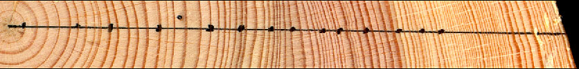

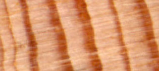
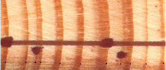
| These two pictures are taken from samples of the demolished house at Bergvik on the island of Nämdö. In real world these two samples are 21 centimetres and 16 centimetres long. They are taken out of two different logs in the house. |
 |  |
|
After grinding and polish these samples have been scanned on an office scanner in 600 dots per inch (dpi).
In full resolution their images look like this on the screen.
Note: For this type of samples you will probably use a scanner resolution between 1600 and 2400 dpi, though in this case the 600 dpi resolution was good enough. |
| This diagram shows the width of each tree ring in both samples. The years are plotted on the horizontal axis and the ringwidths on the vertical axis. If you compare the two curves carefully you will find that there are close points of similarity between them. Though the overall growth rates differ, the variation over time is similar. Bad and good years of growth are reflected at the same time in both curves. |
The red curve corresponds to the green curve in the plain ring widths diagram.
|
As you saw in the ring width diagram, it was difficult to actually identify the similarities
between the ring width curves. Therefore we have done some mathematics on the ring width values. In CDendro, we
name this type of curve processing for a normalization of the curves.
With these normalized curves we then have curves which look much more similar than the plain ring width curves! Dendrochronologists use various algorithms for the normalization. Two algorithms are named after their originators, i.e. Baillie/Pilcher and Hollstein. You can turn on these algorithms within the CDendro program, though the default algorithm of CDendro is "home brewed" and named "Proportion of last two years growth" (Prop2Yrs). It is indeed related to the other algorithms but in many cases found to be more efficient, i.e. it is somewhat better for finding the correct match (ref 1). Proportion of last two years growth normalization: For each ring width value this algorithm calculates a value describing this year's growth as a proportion of the last two years growth. Think of the total growth during the two last years! How much of that (in percent) grew the very last year?
An example: We have the ring widths w1, w2, w3, w4, w5 ... where w1 is the most recent (youngest) ring.
|
|
The process of crossdating implies comparing two curves with each other and trying to find where they fit together.
Here, the red and green curves are shifted stepwise from left to right along the black and blue curves. For each step we try to quantify how well the red and black curves fit together at that point. Let the curves lay over each other. After looking at the mismatch you can set up a score telling how bad it all looks. Then shift the upper curve (drawn on transparent paper) one step (one year) to the right and set up a second score for this mismatch. While stepping and scoring you suddenly see - if you are lucky - a really good match which will give a high score. |
|
Plot your scores, one for each step, and it may look as the picture above.
As you can see there is only one high peak. This occurs when the two curves lay over each other with their very first years overlapping. In real world this means that the two logs were cut the same year. (Not very sensational as they are taken from the same house.) In a book on statistics you will find a description of the correlation coefficient. It can be used as a measure of the covariance between two curves, i.e. how well the curves match each other. We could name it a value showing the quality of the matching. The correlation coefficient is cumbersome to calculate (its algorithm is described below) so you really need a computer for this type of scoring. The plot shown above is actually showing the correlation coefficients calculated from matching our two normalized sample curves shown above. A coefficient value of 1 means that both curves follow each other exactly.
Note: When comparing ring width curves, we do the correlation coefficient mathematics on the normalized curves! When you document a best value from such a correlation calculus, you should also document the normalization method used, as the requirements on the level of the coefficient to acertain a dating, differs somewhat with the normalization method used (ref 1).
|
OverlappingOf course the curves should overlap when we calculate the correlation coefficient. If we shift the curve of one sample so it hangs out a bit to the right of the other curve, it means that we are testing the probability that this sample is younger than the other sample (if later times are to the right in the diagram). It also means that only a part of one curve overlaps the other curve. How much do these curves have to overlap to make a meaningful calculation? My experience is that it should be an overlap of at least 50 years! Anything less than that will give you just a nice coefficient not the basis for a dating.
To make me convinced of a dating, I ask for an overlap of about 80-100 years, a high correlation
coefficient value and a big step to the next best value.
|
TTest/T-scoreTTest values are calculated according to the formula below, where n is the number of overlapping years and c is the correlation coefficient value. |
There is a TTest calculator available within CDendro!
With the click on the "Make corr. analysis" button the computer will check all possible matching positions, and sort out the best ones
and then position the curves relative to each other at the best matching position as shown above.
The Workbench tab will present you with a list of the best matching positions.
Reference curve = Mean value curve
|
When we have several matching curves, we can make a mean value curve of them all and use that curve as a reference when dating new samples.
The picture shows a sample (red and green) compared towards a reference curve (black and blue), created from many trees.
The numbers in black color along the bottom of the diagram show the number of trees involved when calculating the mean ring widths, this is sometimes called "sample depth" or "replication". The numbers in red color represent correlation coefficients calculated for 20 years long segments (blocks) lagged by 10 years. The gray bar above these represents the so called "trend" ("Gleichläufigkeit"), which is either true (gray) or false (no color). The trend is true when growth increases or decreases for both of the reference curve and the sample being compared. |
A reference curve with standard deviations
|
By plotting also the standard deviation around the reference curves you get an idea of what is
an acceptable deviation from the reference curve. The picture above shows many narrow channels
through which the sample curve (the red curve) should best run to make us confident that this is a proper matching.
Standard deviation curves plotted around the reference curve are of great value when inspecting curve matching visually! |
How to calculate ring width mean values? - Detrending
Do not mix up detrending and normalization!
|
Mean values of normalized data are uncomplicated to calculate. Ring width mean values are more complicated to calculate!
The innermost ring widths of a tree are usually the widest rings of that tree, as a young tree grows faster than an old tree. Also - a tree on good soil grows faster than a tree on poor soil! Just adding together ring widths of a certain year and then dividing by the number of trees, is not a good strategy if we want a mean value that mirrors the growth conditions of that year. Then tree rings from then young trees would dominate the calculations. Detrending of a ring width curve is the process of modifying that curve to remove the effects of tree aging from the ring width data. It also includes a scaling of the ring width curve to compensate for the effects of rich or poor soil. In principle, the detrending of a ring width curve is done by dividing each ring width value with the mean ring width value of the whole tree. This calculation makes growth curves from different trees comparable though their mean ring width values differ greatly because of different growth conditions. |
|
If the innermost rings of a tree are wider than the outer rings, then a negative exponential curve is fitted as a detrending curve to the ring width curve. Each ring width is then divided by the corresponding value of the detrending curve. This will compensate for the decrease in growth related to aging. |
| When it is not possible to fit a negative exponential curve to the growth curve, the growth curve is divided by the mean value of the curve, which corresponds to a horizontal straight line. This is problematic if a tree was suppressed by surrounding trees when it was young - resulting in slow growth - and then later started to grow faster. |
| In such a case it may be better to crop the curve and remove the ring widths of the earliest years of the tree. An alternative would be to have a detrending curve that adapts better to the curvature of the original tree ring curve. For some more information, see the section on "Detrending", ref 2. |
|
References:
1. AXELSON, T.: "What is a good TTest value to ensure a dating?" 2. Detrending |